Code
library(tidyverse)
library(broom)
library(scales)
library(ggdag)library(tidyverse)
library(broom)
library(scales)
library(ggdag)Draw a DAG that maps out how all the columns you care about are related.
Regression discontinuity designs are also based on context instead of models, so the DAG is pretty simple. We’ll keep with our mosquito net example and pretend that families that earn less than $450 a week qualify for a free net. Here’s the DAG:
rdd_dag <- dagify(
  mal ~ net + inc,
  net ~ cut,
  cut ~ inc,
  coords = list(
    x = c(mal = 4, net = 1, inc = 3, cut = 2),
    y = c(mal = 1, net = 1, inc = 2, cut = 1.75)
  )
)

ggdag(rdd_dag) +
  theme_dag()
Specify how those nodes are measured.
Here’s how we’ll measure these nodes:
Malaria risk: scale from 0–100, mostly around 60, but ranging from 30ish to 90ish. Best to use a Beta distribution.
Net use: binary 0/1, TRUE/FALSE variable. This is technically binomial, but we don’t need to simulate it since it will only happen for people who below the cutoff.
Income: weekly income, measured in dollars, mostly around 500 ± 300. Best to use a normal distribution.
Cutoff: binary 0/1, below/above $450 variable. This is technically binomial, but we don’t need to simulate it since it is entirely based on income.
Specify the relationships between the nodes based on the DAG equations.
There are three models in the DAG:
cut ~ inc: Being above or below the cutpoint is determined by income. We know the cutoff is 450, so we just make an indicator showing if people are below that.
net ~ cut: Net usage is determined by the cutpoint. If people are below the cutpoint, they’ll use a net; if not, they won’t. We can build in noncompliance here if we want and use fuzzy regression discontinuity. For the sake of this example, we’ll do it both ways, just so you can see both sharp and fuzzy synthetic data.
mal ~ net + inc: Malaria risk is determined by both net usage and income. It’s also determined by lots of other things (age, education, city, etc.), but we don’t need to include those in the DAG because we’re using RDD to say that we have good treatment and control groups right around the cutoff.
We’ll pretend that a 1 dollar increase in income is associated with a drop in risk of 0.01, and that using a mosquito net causes a decrease of 10 points on average. That’s our causal effect.
Generate random columns that stand alone. Generate related columns using regression math. Consider adding random noise. This is an entirely trial and error process until you get numbers that look good. Rely heavily on plots as you try different coefficients and parameters. Optionally rescale any columns that go out of reasonable bounds. If you rescale, you’ll need to tinker with the coefficients you used since the final effects will also get rescaled.
Let’s fake some data! Heavily annotated code below:
I include both sharp and fuzzy versions of the treatment (net usage here) for illustration. You shouldn’t do this with your data. You need to decide if your treatment is fuzzy or sharp and use the corresponding approach.
# Make this randomness consistent
set.seed(1234)

# Simulate 5441 people (we need a lot bc we're throwing most away)
n_people <- 5441

rdd_data <- tibble(
  # Make an ID column (not necessary, but nice to have)
  id = 1:n_people,
  # Generate income variable: normal, 500 ± 300
  income = rnorm(n_people, mean = 500, sd = 75)
) |>
  # Generate cutoff variable
  mutate(below_cutoff = ifelse(income < 450, TRUE, FALSE)) |>
  # Generate net variable. We'll make two: one that's sharp and has perfect
  # compliance, and one that's fuzzy
  # Here's the sharp one. It's easy. If you're below the cutoff you use a net.
  mutate(net_sharp = ifelse(below_cutoff == TRUE, TRUE, FALSE)) |>
  # Here's the fuzzy one, which is a little trickier. If you're far away from
  # the cutoff, you follow what you're supposed to do (like if your income is
  # 800, you don't use the program; if your income is 200, you definitely use
  # the program). But if you're close to the cutoff, we'll pretend that there's
  # an 80% chance that you'll do what you're supposed to do.
  mutate(
    net_fuzzy = case_when(
      # If your income is between 450 and 500, there's a 20% chance of using the program
      income >= 450 & income <= 500 ~
        sample(c(TRUE, FALSE), n_people, replace = TRUE, prob = c(0.2, 0.8)),
      # If your income is above 500, you definitely don't use the program
      income > 500 ~ FALSE,
      # If your income is between 400 and 450, there's an 80% chance of using the program
      income < 450 & income >= 400 ~
        sample(c(TRUE, FALSE), n_people, replace = TRUE, prob = c(0.8, 0.2)),
      # If your income is below 400, you definitely use the program
      income < 400 ~ TRUE
    )
  ) |>
  # Finally we can make the malaria risk score, based on income, net use, and
  # random noise. We'll make two outcomes: one using the sharp net use and one
  # using the fuzzy net use. They have the same effect built in, we just have to
  # use net_sharp and net_fuzzy separately.
  mutate(malaria_risk_base = rbeta(n_people, shape1 = 4, shape2 = 5) * 100) |>
  # Make the sharp version. There's really a 10 point decrease, but because of
  # rescaling, we use 15. I only chose 15 through lots of trial and error (i.e.
  # I used -11, ran the RDD model, and the effect was too small; I used -20, ran
  # the model, and the effect was too big; I kept changing numbers until landing
  # on -15). Risk also goes down as income increases.
  mutate(
    malaria_effect_sharp = (-15 * net_sharp) + (-0.01 * income),
    malaria_risk_sharp = malaria_risk_base +
      malaria_effect_sharp +
      rnorm(n_people, 0, sd = 3),
    malaria_risk_sharp = rescale(malaria_risk_sharp, to = c(5, 70))
  ) |>
  # Do the same thing, but with net_fuzzy
  mutate(
    malaria_effect_fuzzy = (-15 * net_fuzzy) + (-0.01 * income),
    malaria_risk_fuzzy = malaria_risk_base +
      malaria_effect_fuzzy +
      rnorm(n_people, 0, sd = 3),
    malaria_risk_fuzzy = rescale(malaria_risk_fuzzy, to = c(5, 70))
  ) |>
  # Make a version of income that's centered at the cutpoint
  mutate(income_centered = income - 450)

head(rdd_data)
## # A tibble: 6 × 11
##      id income below_cutoff net_sharp net_fuzzy malaria_risk_base malaria_effect_sharp malaria_risk_sharp malaria_effect_fuzzy malaria_risk_fuzzy income_centered
##   <int>  <dbl> <lgl>        <lgl>     <lgl>                 <dbl>                <dbl>              <dbl>                <dbl>              <dbl>           <dbl>
## 1     1   409. TRUE         TRUE      FALSE                  56.5               -19.1                38.0                -4.09               47.5           -40.5
## 2     2   521. FALSE        FALSE     FALSE                  26.1                -5.21               28.6                -5.21               27.6            70.8
## 3     3   581. FALSE        FALSE     FALSE                  84.4                -5.81               64.7                -5.81               65.5           131.
## 4     4   324. TRUE         TRUE      TRUE                   32.9               -18.2                25.9               -18.2                23.4          -126.
## 5     5   532. FALSE        FALSE     FALSE                  53.1                -5.32               46.5                -5.32               44.3            82.2
## 6     6   538. FALSE        FALSE     FALSE                  45.7                -5.38               43.2                -5.38               40.2            88.0
Verify all relationships with plots and models.
Is there a cutoff in the running variable when we use the sharp net variable? Yep!
ggplot(rdd_data, aes(x = income, y = net_sharp, color = below_cutoff)) +
  geom_vline(xintercept = 450) +
  geom_point(alpha = 0.3, position = position_jitter(width = NULL, height = 0.2)) +
  guides(color = "none")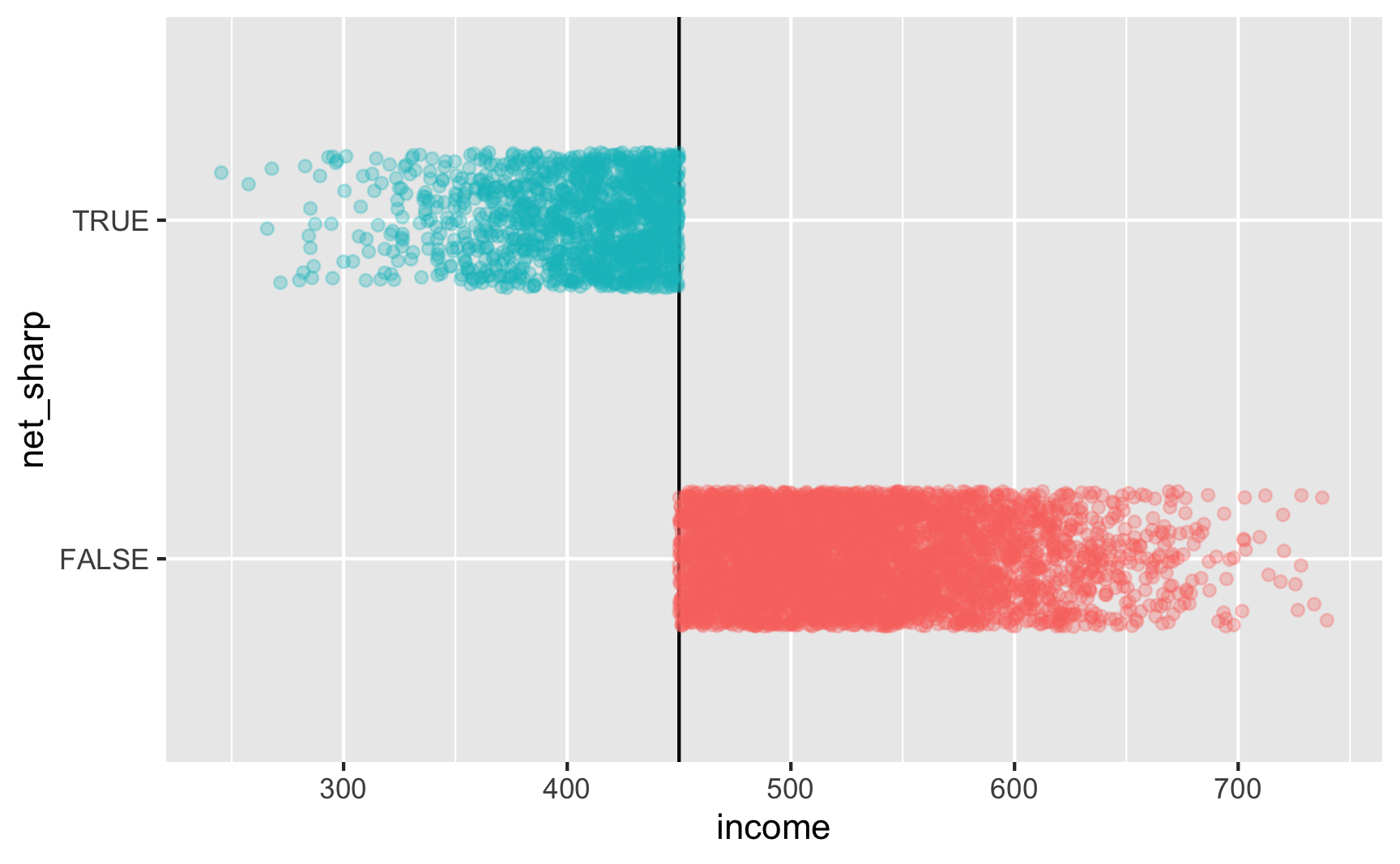
Is there a cutoff in the running variable when we use the fuzzy net variable? Yep! There are some richer people using the program and some poorer people not using it.
ggplot(rdd_data, aes(x = income, y = net_fuzzy, color = below_cutoff)) +
  geom_vline(xintercept = 450) +
  geom_point(alpha = 0.3, position = position_jitter(width = NULL, height = 0.2)) +
  guides(color = "none")
Try it out!
Let’s test it! For sharp RDD we need to use this model:
\[ \text{Malaria risk} = \beta_0 + \beta_1 \text{Income}_\text{centered} + \beta_2 \text{Net} + \varepsilon \]
We’ll use a bandwidth of ±$50, because why not. In real life you’d be more careful about bandwidth selection (or use rdbwselect() from the {rdrobust} package to find the optimal bandwidth)
ggplot(rdd_data, aes(x = income, y = malaria_risk_sharp, color = net_sharp)) +
  geom_vline(xintercept = 450) +
  geom_point(alpha = 0.2, size = 0.5) +
  # Add lines for the full range
  geom_smooth(data = filter(rdd_data, income_centered <= 0),
              method = "lm", se = FALSE, size = 1, linetype = "dashed") +
  geom_smooth(data = filter(rdd_data, income_centered > 0),
              method = "lm", se = FALSE, size = 1, linetype = "dashed") +
  # Add lines for bandwidth = 50
  geom_smooth(data = filter(rdd_data, income_centered >= -50 & income_centered <= 0),
              method = "lm", se = FALSE, size = 2) +
  geom_smooth(data = filter(rdd_data, income_centered > 0 & income_centered <= 50),
              method = "lm", se = FALSE, size = 2) +
  theme(legend.position = "bottom")
## Warning: Using `size` aesthetic for lines was deprecated in ggplot2 3.4.0.
## ℹ Please use `linewidth` instead.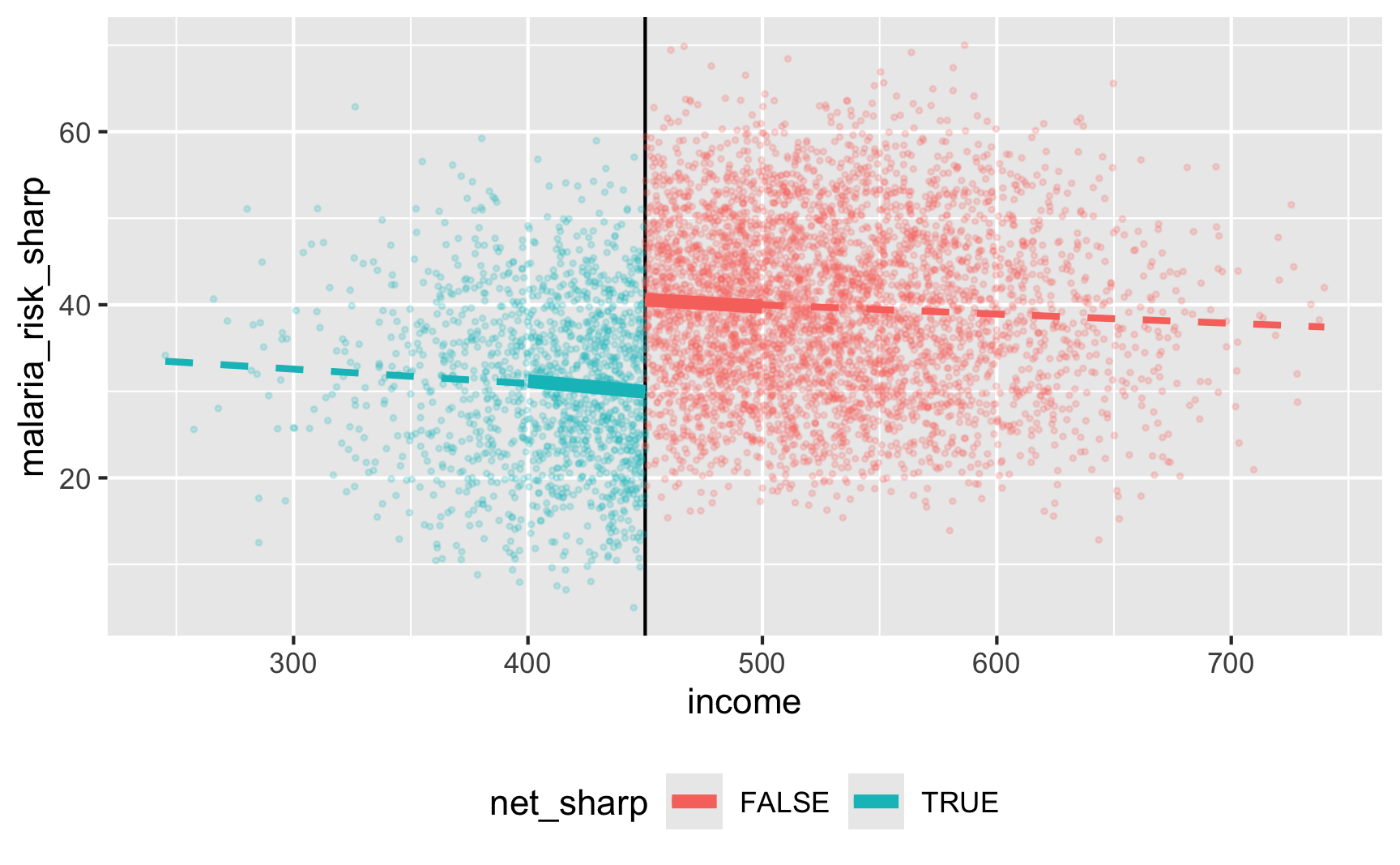
model_sharp <- lm(
  malaria_risk_sharp ~ income_centered + net_sharp,
  data = filter(rdd_data, income_centered >= -50 & income_centered <= 50)
)
tidy(model_sharp)
## # A tibble: 3 × 5
##   term            estimate std.error statistic  p.value
##   <chr>              <dbl>     <dbl>     <dbl>    <dbl>
## 1 (Intercept)      40.7       0.462      88.1  0
## 2 income_centered  -0.0197    0.0144     -1.37 1.72e- 1
## 3 net_sharpTRUE   -10.6       0.815     -13.0  1.67e-37
There’s an effect! For people in the bandwidth, the local average treatment effect of nets is a 10.6 point reduction in malaria risk.
Let’s check if it works with the fuzzy version where there are noncompliers:
ggplot(rdd_data, aes(x = income, y = malaria_risk_fuzzy, color = net_fuzzy)) +
  geom_vline(xintercept = 450) +
  geom_point(alpha = 0.2, size = 0.5) +
  # Add lines for the full range
  geom_smooth(data = filter(rdd_data, income_centered <= 0),
              method = "lm", se = FALSE, size = 1, linetype = "dashed") +
  geom_smooth(data = filter(rdd_data, income_centered > 0),
              method = "lm", se = FALSE, size = 1, linetype = "dashed") +
  # Add lines for bandwidth = 50
  geom_smooth(data = filter(rdd_data, income_centered >= -50 & income_centered <= 0),
              method = "lm", se = FALSE, size = 2) +
  geom_smooth(data = filter(rdd_data, income_centered > 0 & income_centered <= 50),
              method = "lm", se = FALSE, size = 2) +
  theme(legend.position = "bottom")
There’s a gap, but it’s hard to measure since there are noncompliers on both sides. We can deal with the noncompliance if we use above/below the cutoff as an instrument (see the fuzzy regression discontinuity guide for a complete example). We should run this set of models:
\[ \begin{aligned} \widehat{\text{Net}} &= \gamma_0 + \gamma_1 \text{Income}_{\text{centered}} + \gamma_2 \text{Below 450} + \omega \\\\ \text{Malaria risk} &= \beta_0 + \beta_1 \text{Income}\_{\text{centered}} + \beta_2 \widehat{\text{Net}} + \epsilon \end{aligned} \]
Instead of doing these two stages by hand (ugh), we’ll do the 2SLS regression with the iv_robust() function from the {estimatr} package:
library(estimatr)

model_fuzzy <- iv_robust(
  malaria_risk_fuzzy ~ income_centered + net_fuzzy | income_centered + below_cutoff,
  data = filter(rdd_data, income_centered >= -50 & income_centered <= 50)
)
tidy(model_fuzzy)
##              term  estimate std.error statistic   p.value  conf.low conf.high   df            outcome
## 1     (Intercept)  40.73241   0.69045    58.994 0.000e+00  39.37843 42.086402 2220 malaria_risk_fuzzy
## 2 income_centered  -0.01921   0.01423    -1.350 1.772e-01  -0.04711  0.008696 2220 malaria_risk_fuzzy
## 3   net_fuzzyTRUE -11.21929   1.31033    -8.562 2.034e-17 -13.78889 -8.649700 2220 malaria_risk_fuzzy
The effect is slightly larger now (−11.2), but that’s because we are looking at a doubly local ATE: compliers in the bandwidth. But still, it’s close to −10, so that’s good. And we could probably get it closer if we did other mathy shenanigans like adding squared and cubed terms or using nonparametric estimation with rdrobust() in the {rdrobust} package.
Save the data.
The data works, so let’s get rid of the intermediate columns we don’t need and save it as a CSV file. We’ll make two separate CSV files for fuzzy and sharp, just because.
rdd_data_final_sharp <- rdd_data |>
  select(id, income, net = net_sharp, malaria_risk = malaria_risk_sharp)
head(rdd_data_final_sharp)
## # A tibble: 6 × 4
##      id income net   malaria_risk
##   <int>  <dbl> <lgl>        <dbl>
## 1     1   409. TRUE          38.0
## 2     2   521. FALSE         28.6
## 3     3   581. FALSE         64.7
## 4     4   324. TRUE          25.9
## 5     5   532. FALSE         46.5
## 6     6   538. FALSE         43.2

rdd_data_final_fuzzy <- rdd_data |>
  select(id, income, net = net_fuzzy, malaria_risk = malaria_risk_fuzzy)
head(rdd_data_final_fuzzy)
## # A tibble: 6 × 4
##      id income net   malaria_risk
##   <int>  <dbl> <lgl>        <dbl>
## 1     1   409. FALSE         47.5
## 2     2   521. FALSE         27.6
## 3     3   581. FALSE         65.5
## 4     4   324. TRUE          23.4
## 5     5   532. FALSE         44.3
## 6 6 538. FALSE 40.2# Save data
write_csv(rdd_data_final_sharp, "data/rdd_sharp.csv")
write_csv(rdd_data_final_fuzzy, "data/rdd_fuzzy.csv")