Code
library(tidyverse)
library(broom)
library(scales)
library(ggdag)library(tidyverse)
library(broom)
library(scales)
library(ggdag)Draw a DAG that maps out how all the columns you care about are related.
RCTs are great because they make DAGs really easy! In a well-randomized RCT, you get to delete all arrows going into the treatment node in a DAG. We’ll stick with the same mosquito net situation we just used, but make it randomized:
rct_dag <- dagify(
  mal ~ net + inc + hlth,
  hlth ~ inc,
  coords = list(
    x = c(mal = 4, net = 1, inc = 2, hlth = 3),
    y = c(mal = 1, net = 1, inc = 2, hlth = 2)
  )
)

ggdag(rct_dag) +
  theme_dag()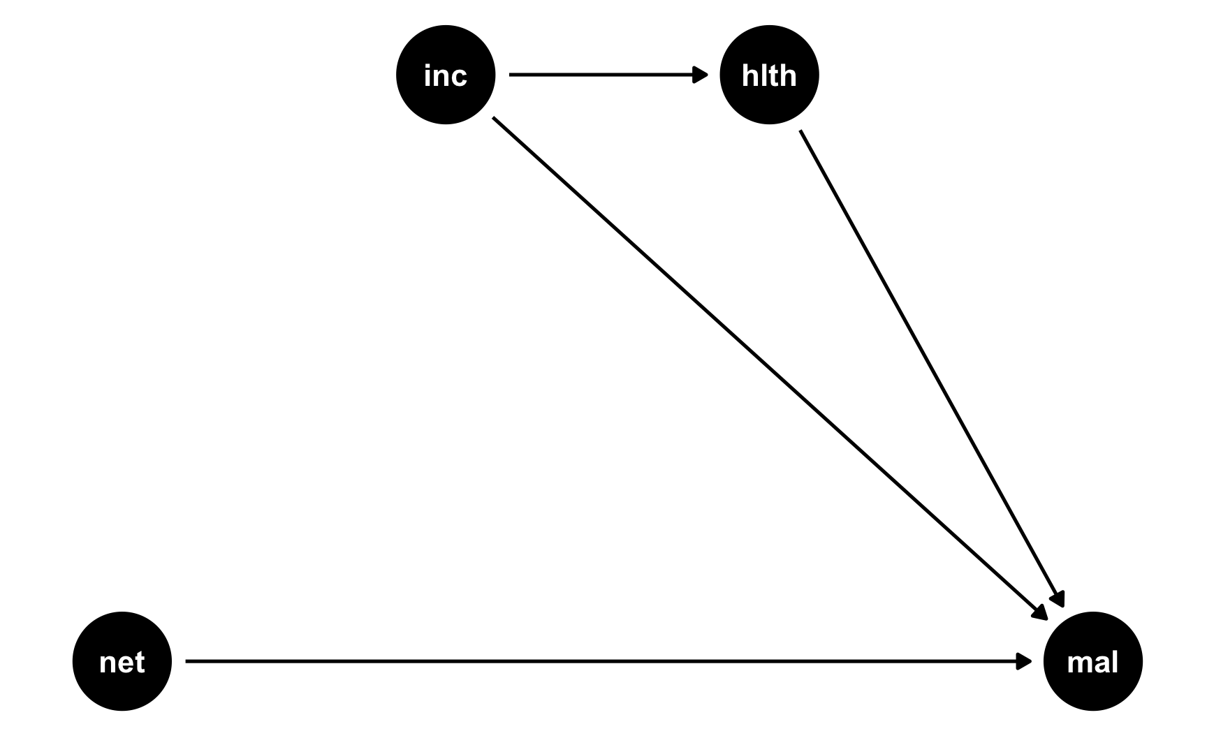
Specify how those nodes are measured.
We’ll measure these nodes the same way as before:
Malaria risk: scale from 0–100, mostly around 40, but ranging from 10ish to 80ish. Best to use a Beta distribution.
Net use: binary 0/1, TRUE/FALSE variable, where 50% of people use nets. Best to use a binomial distribution.
Income: weekly income, measured in dollars, mostly around 500 ± 300. Best to use a normal distribution.
Health: scale from 0–100, mostly around 70, but ranging from 50ish to 100. Best to use a Beta distribution.
Specify the relationships between the nodes based on the DAG equations.
This is where RCTs are great. Because we removed all the arrows going into net, we don’t need to build any relationships that influence net use. Net use is randomized! We don’t need to make strange “bed net scores” and give people boosts according to income or health or anything. There are only two models in this DAG:
hlth ~ inc: Income influences health. We’ll assume that every 10 dollars/week is associated with a 1 point increase in health (so a 1 dollar incrrease is associated with a 0.02 point increase in health)
mal ~ net + inc + hlth: Net use, income, and health all have an effect on the risk of malaria. We’ll say that a 1 dollar increase in income is associated with a decrease in risk, a 1 point increase in health is associated with a decrease in risk, and using a net is associated with a 15 point decrease in risk. That’s the casual effect we’re building in to the DAG.
Generate exogenous columns that stand alone. Generate endogenous columns using regression math. Consider adding random noise. This is an entirely trial and error process until you get numbers that look good. Rely heavily on plots as you try different coefficients and parameters. Optionally rescale any columns that go out of reasonable bounds. If you rescale, you’ll need to tinker with the coefficients you used since the final effects will also get rescaled.
Let’s make this data. It’ll be a lot easier than the full DAG we did before. Again, I’ll comment the code below so you can see what’s happening at each step.
# Make this randomness consistent
set.seed(1234)

# Simulate 793 people (just for fun)
n_people <- 793

rct_data <- tibble(
  # Make an ID column (not necessary, but nice to have)
  id = 1:n_people,
  # Generate income variable: normal, 500 ± 300
  income = rnorm(n_people, mean = 500, sd = 75)
) |>
  # Generate health variable: beta, centered around 70ish
  mutate(
    health_base = rbeta(n_people, shape1 = 7, shape2 = 4) * 100,
    # Health increases by 0.02 for every dollar in income
    health_income_effect = income * 0.02,
    # Make the final health score and add some noise
    health = health_base +
      health_income_effect +
      rnorm(n_people, mean = 0, sd = 3),
    # Rescale so it doesn't go above 100
    health = rescale(health, to = c(min(health), 100))
  ) |>
  # Randomly assign people to use a net (this is nice and easy!)
  mutate(net = rbinom(n_people, 1, 0.5)) |>
  # Finally generate a malaria risk variable based on income, health, net use,
  # and random noise
  mutate(
    malaria_risk_base = rbeta(n_people, shape1 = 4, shape2 = 5) * 100,
    # Risk goes down by 10 when using a net. Because we rescale things,
    # though, we have to make the effect a lot bigger here so it scales
    # down to -10. Risk also decreases as health and income go up. I played
    # with these numbers until they created reasonable coefficients.
    malaria_effect = (-35 * net) + (-1.9 * health) + (-0.1 * income),
    # Make the final malaria risk score and add some noise
    malaria_risk = malaria_risk_base +
      malaria_effect +
      rnorm(n_people, 0, sd = 3),
    # Rescale so it doesn't go below 0,
    malaria_risk = rescale(malaria_risk, to = c(5, 70))
  )

# Look at all these columns!
head(rct_data)
## # A tibble: 6 × 9
##      id income health_base health_income_effect health   net malaria_risk_base malaria_effect malaria_risk
##   <int>  <dbl>       <dbl>                <dbl>  <dbl> <int>             <dbl>          <dbl>        <dbl>
## 1     1   409.        57.2                 8.19   61.3     1              37.4          -192.         35.1
## 2     2   521.        63.3                10.4    69.4     0              33.0          -184.         37.6
## 3     3   581.        61.8                11.6    71.9     1              36.4          -230.         24.4
## 4     4   324.        42.2                 6.48   45.5     1              52.7          -154.         52.8
## 5     5   532.        72.1                10.6    78.5     1              41.9          -237.         23.6
## 6     6   538.        82.0                10.8    89.1     0              46.6          -223.         29.9
Verify all relationships with plots and models.
Income still looks like it’s associated with health (which isn’t surprising, since it’s the same code we used for the full DAG earlier):
ggplot(rct_data, aes(x = income, y = health)) +
  geom_point() +
  geom_smooth(method = "lm")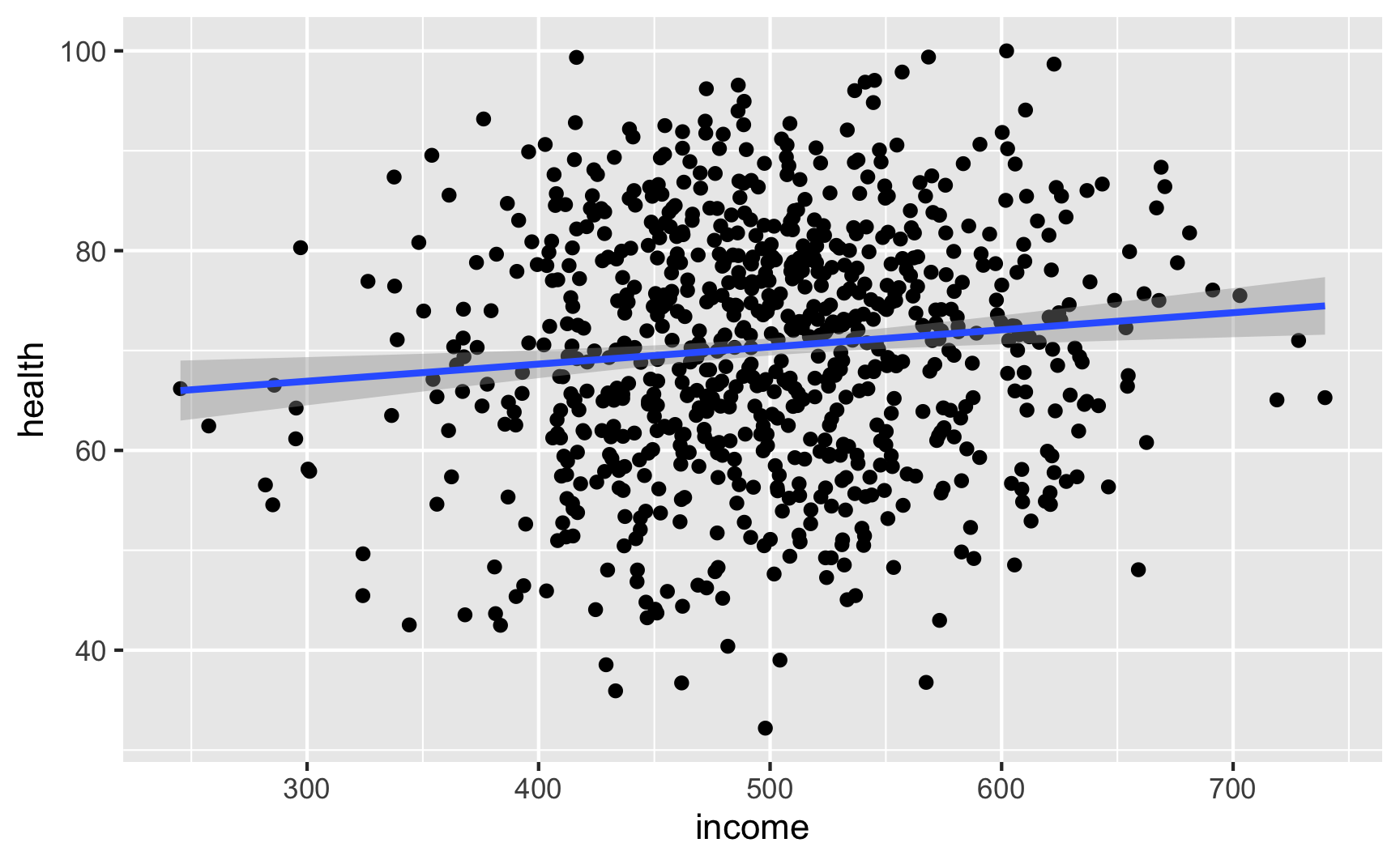
lm(health ~ income, data = rct_data) |> tidy()
## # A tibble: 2 × 5
##   term        estimate std.error statistic  p.value
##   <chr>          <dbl>     <dbl>     <dbl>    <dbl>
## 1 (Intercept)  61.8      2.92        21.1  5.20e-79
## 2 income        0.0171   0.00580      2.96 3.21e- 3
Try it out!
Is the effect in there? With an RCT, all we really need to do is compare the outcome across treatment and control groups—because there’s no confounding, we don’t need to control for anything. Ordinarily we should check for balance across characteristics like health and income (and maybe generate other demographic columns) like we did in the RCT example, but we’ll skip all that here since we’re just checking to see if the effect is there.
It looks like using nets causes an average decrease of 10 risk points. Great!
# Correct RCT-based ATE
model_rct <- lm(malaria_risk ~ net, data = rct_data)
tidy(model_rct)
## # A tibble: 2 × 5
##   term        estimate std.error statistic  p.value
##   <chr>          <dbl>     <dbl>     <dbl>    <dbl>
## 1 (Intercept)     40.8     0.463      88.0 0
## 2 net            -10.2     0.653     -15.7 2.22e-48
Just for fun, if we control for health and income, we’ll get basically the same effect, since they don’t actualy confound the relationship and don’t really explain anything useful.
# Controlling for stuff even though we don't need to
model_rct_controls <- lm(malaria_risk  ~ net + health + income, data = rct_data)
tidy(model_rct_controls)
## # A tibble: 4 × 5
##   term        estimate std.error statistic   p.value
##   <chr>          <dbl>     <dbl>     <dbl>     <dbl>
## 1 (Intercept)  97.7      1.45         67.3 0
## 2 net         -10.8      0.344       -31.3 2.27e-140
## 3 health       -0.586    0.0140      -41.8 1.67e-202
## 4 income       -0.0310   0.00230     -13.5 1.75e- 37
Save the data.
The data works, so let’s get rid of the intermediate columns we don’t need and save it as a CSV file.
# In the end, all we need is id, income, health, net, and malaria risk:
rct_data_final <- rct_data |>
  select(id, income, health, net, malaria_risk)
head(rct_data_final)
## # A tibble: 6 × 5
##      id income health   net malaria_risk
##   <int>  <dbl>  <dbl> <int>        <dbl>
## 1     1   409.   61.3     1         35.1
## 2     2   521.   69.4     0         37.6
## 3     3   581.   71.9     1         24.4
## 4     4   324.   45.5     1         52.8
## 5     5   532.   78.5     1         23.6
## 6 6 538. 89.1 0 29.9# Save it as a CSV file
write_csv(rct_data_final, "data/bed_nets_rct.csv")