Code
library(tidyverse)
library(broom)
library(scales)
library(ggdag)library(tidyverse)
library(broom)
library(scales)
library(ggdag)Draw a DAG that maps out how all the columns you care about are related.
As with diff-in-diff and regression discontinuity, instrumental variables are a circumstantial approach to causal inference and thus don’t require complicated models (but you can still add control variables!), so their DAGs are simpler. Once again we’ll look at the effect of mosquito nets on malaria risk, but this time we’ll say that we cannot possibly measure all the confounding factors between net use and malaria risk, so we’ll use an instrument to extract the exogeneity from net use.
As we talked about in Session 11, good plausible instruments are hard to find: they have to cause bed net use and not be related to malaria risk except through bed net use.
For this example, we’ll pretend that free bed nets are distributed from town halls around the country. We’ll use “distance to town hall” as our instrument, since it could arguably maybe work perhaps. Being closer to a town hall makes you more likely to use a net, but being closer to a town halls doesn’t make put you at higher or lower risk for malaria on its own—it does that only because it changes your likelihood of getting a net.
This is where the story for the instrument falls apart, actually; in real life, if you live far away from a town hall, you probably live further from health services and live in more rural places with worse mosquito abatement policies, so you’re probably at higher risk of malaria. It’s probably a bad instrument, but just go with it.
Here’s the DAG:
iv_dag <- dagify(
  mal ~ net + U,
  net ~ dist + U,
  coords = list(
    x = c(mal = 4, net = 2, U = 3, dist = 1),
    y = c(mal = 1, net = 1, U = 2, dist = 1.5)
  ),
  latent = "U"
)

ggdag_status(iv_dag) +
  guides(color = "none") +
  theme_dag()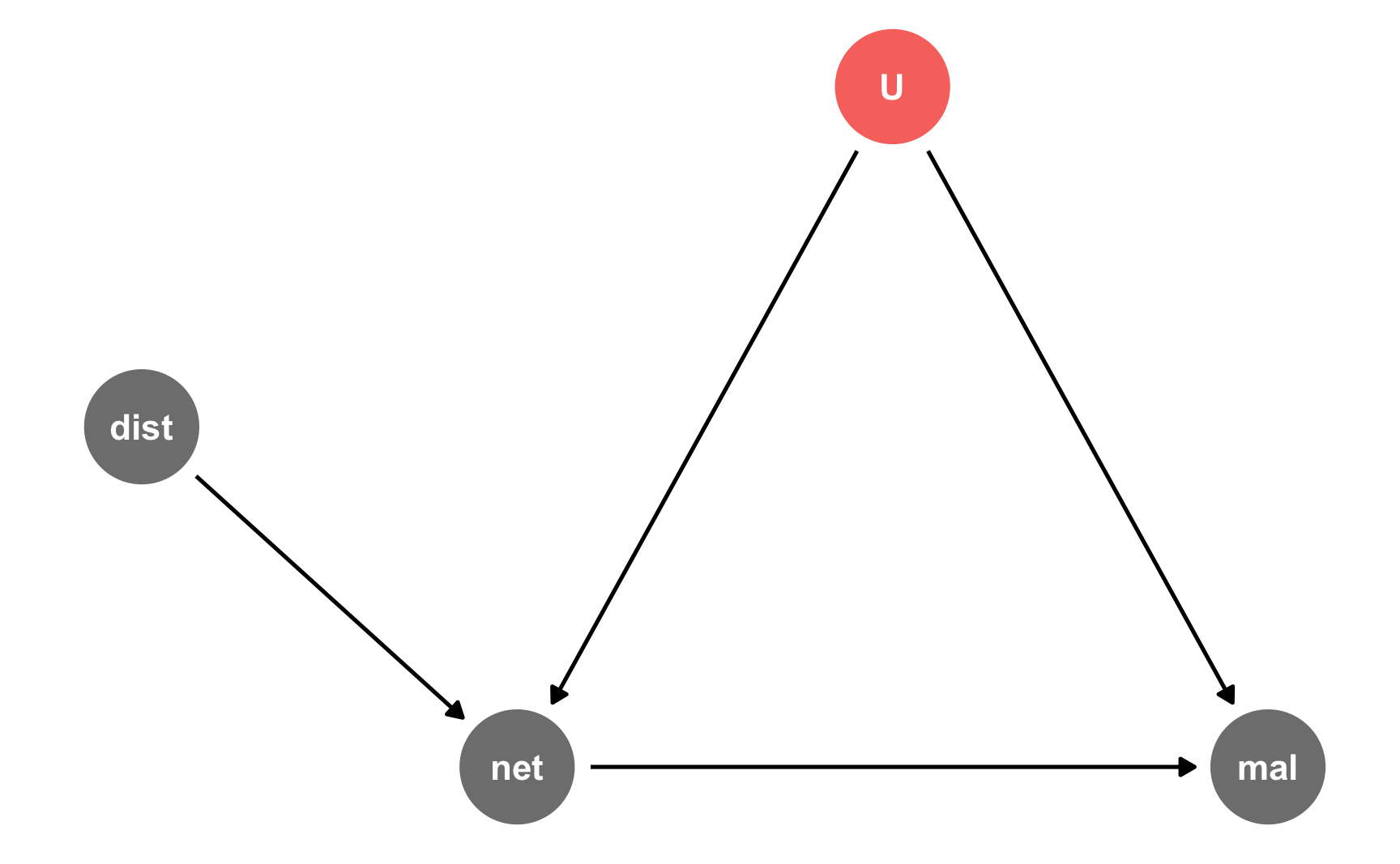
Specify how those nodes are measured.
Here’s how we’ll measure these nodes:
Malaria risk: scale from 0–100, mostly around 60, but ranging from 30ish to 90ish. Best to use a Beta distribution.
Net use: binary 0/1, TRUE/FALSE variable. However, since we want to use other variables that increase the likelihood of using a net, we’ll do some cool tricky stuff with a bed net score, like we did in the observational DAG example earlier.
Distance: distance to nearest town hall, measured in kilometers, mostly around 3, with a left skewed long tail (i.e. most people live fairly close, some people live far away). Best to use a Beta distribution (to get the skewed shape) that we then rescale.
Unobserved: who knows?! There are a lot of unknown confounders. We could generate columns like income, age, education, and health, make them mathematically related to malaria risk and net use, and then throw those columns away in the final data so they’re unobserved. That would be fairly easy and intuitive.
For the sake of simplicity here, we’ll make a column called “risk factors,” kind of like we did with the “ability” column in the instrumental variables example—it’s a magical column that is unmeasurable, but it’ll open a backdoor path between net use and malaria risk and thus create endogeneity. It’ll be normally distributed around 50, with a standard deviation of 25.
Specify the relationships between the nodes based on the DAG equations.
There are two models in the DAG:
net ~ dist + U: Net usage is determined by both distance and our magical unobserved risk factor column. Net use is technically binomial, but in order to change the likelihood of net use based on distance to town hall and unobserved stuff, we’ll do the fancy tricky stuff we did in the observational DAG section above: we’ll create a bed net score, increase or decrease that score based on risk factors and distance, scale that score to a 0-1 scale of probabilities, and then draw a binomial 0/1 outcome using those probabilities.
We’ll say that a one kilometer increase in the distance to a town halls reduces the bed net score and a one point increase in risk factors reduces the bed net score.
mal ~ net + U: Malaria risk is determined by both net usage and unkown stuff, or the magical column we’re calling “risk factors.” We’ll say that a one point increase in risk factors increases malaria risk, and that using a mosquito net causes a decrease of 10 points on average. That’s our causal effect.
Generate random columns that stand alone. Generate related columns using regression math. Consider adding random noise. This is an entirely trial and error process until you get numbers that look good. Rely heavily on plots as you try different coefficients and parameters. Optionally rescale any columns that go out of reasonable bounds. If you rescale, you’ll need to tinker with the coefficients you used since the final effects will also get rescaled.
Fake data time! Here’s some heavily annotated code:
# Make this randomness consistent
set.seed(1234)

# Simulate 1578 people (just for fun)
n_people <- 1578

iv_data <- tibble(
  # Make an ID column (not necessary, but nice to have)
  id = 1:n_people,
  # Generate magical unobserved risk factor variable: normal, 500 ± 300
  risk_factors = rnorm(n_people, mean = 100, sd = 25),
  # Generate distance to town hall variable
  distance = rbeta(n_people, shape1 = 1, shape2 = 4)
) |>
  # Scale up distance to be 0.1-15 instead of 0-1
  mutate(distance = rescale(distance, to = c(0.1, 15))) |>
  # Generate net variable based on distance, risk factors, and random noise
  # Note: These -40 and -2 effects are entirely made up and I got them through a
  # lot of trial and error and rerunning this stupid chunk dozens of times
  mutate(
    net_score = 0 +
      (-40 * distance) + # Distance effect
      (-2 * risk_factors) + # Risk factor effect
      rnorm(n_people, mean = 0, sd = 50), # Random noise
    net_probability = rescale(net_score, to = c(0.15, 1)),
    # Randomly generate a 0/1 variable using that probability
    net = rbinom(n_people, 1, net_probability)
  ) |>
  # Generate malaria risk variable based on net use, risk factors, and random noise
  mutate(
    malaria_risk_base = rbeta(n_people, shape1 = 7, shape2 = 5) * 100,
    # We're aiming for a -10 net effect, but need to boost it because of rescaling
    malaria_effect = (-20 * net) + (0.5 * risk_factors),
    # Make the final malaria risk score
    malaria_risk = malaria_risk_base + malaria_effect,
    # Rescale so it doesn't go below 0
    malaria_risk = rescale(malaria_risk, to = c(5, 80))
  )
iv_data
## # A tibble: 1,578 × 9
##       id risk_factors distance net_score net_probability   net malaria_risk_base malaria_effect malaria_risk
##    <int>        <dbl>    <dbl>     <dbl>           <dbl> <int>             <dbl>          <dbl>        <dbl>
##  1     1         69.8    3.98      -202.           0.766     1              71.1           14.9         36.5
##  2     2        107.     2.14      -284.           0.686     1              75.4           33.5         49.5
##  3     3        127.     5.47      -469.           0.505     0              57.4           63.6         56.4
##  4     4         41.4    9.61      -414.           0.558     0              37.2           20.7         20.4
##  5     5        111.     4.66      -376.           0.596     0              38.5           55.4         40.9
##  6     6        113.     2.29      -284.           0.686     1              75.7           36.3         51.3
##  7     7         85.6    0.922     -215.           0.753     0              28.7           42.8         28.2
##  8     8         86.3   12.5       -608.           0.368     1              50.6           23.2         29.4
##  9     9         85.9    3.11      -267.           0.703     1              38.4           22.9         22.4
## 10    10         77.7    1.35      -157.           0.810     1              69.1           18.9         37.6
## # ℹ 1,568 more rows
Verify all relationships with plots and models.
Is there a relationship between unobserved risk factors and malaria risk? Yep.
ggplot(iv_data, aes(x = risk_factors, y = malaria_risk)) +
  geom_point(aes(color = as.factor(net))) +
  geom_smooth(method = "lm")
Is there a relationship between distance to town hall and net use? Yeah, those who live further away are less likely to use a net.
ggplot(iv_data, aes(x = distance, fill = as.factor(net))) +
  geom_density(alpha = 0.7)
Is there a relationship between net use and malaria risk? Haha, yeah, that’s a huge highly significant effect. Probably too perfect. We could increase those error bars if we tinker with some of the numbers in the code, but for the sake of this example, we’ll leave them like this.
ggplot(iv_data, aes(x = as.factor(net), y = malaria_risk, color = as.factor(net))) +
  stat_summary(geom = "pointrange", fun.data = "mean_se")
Try it out!
Cool, let’s see if this works. Remember, we can’t actually use the risk_factors column in real life, but we will here just to make sure the effect we built in exists. Here’s the true effect, where using a net causes a decrease of 10.9 malaria risk points
model_forbidden <- lm(malaria_risk ~ net + risk_factors, data = iv_data)
tidy(model_forbidden)
## # A tibble: 3 × 5
##   term         estimate std.error statistic   p.value
##   <chr>           <dbl>     <dbl>     <dbl>     <dbl>
## 1 (Intercept)    20.6     0.873        23.6 6.98e-106
## 2 net           -10.8     0.400       -27.1 3.93e-133
## 3 risk_factors    0.283   0.00788      35.9 1.16e-206
Since we can’t actually use that column, we’ll use distance to town hall as an instrument. We should run this set of models:
\[ \begin{aligned} \widehat{\text{Net}} &= \gamma_0 + \gamma_1 \text{Distance to town hall} + \omega \\\\ \text{Malaria risk} &= \beta_0 + \beta_1 \widehat{\text{Net}} + \epsilon \end{aligned} \]
We’ll run this 2SLS model with the iv_robust() function from the {estimatr} package:
library(estimatr)

model_iv <- iv_robust(malaria_risk ~ net | distance, data = iv_data)
tidy(model_iv)
##          term estimate std.error statistic    p.value conf.low conf.high   df      outcome
## 1 (Intercept)   47.202     1.576     29.95 2.344e-156    44.11    50.294 1576 malaria_risk
## 2         net   -8.236     2.474     -3.33  8.889e-04   -13.09    -3.385 1576 malaria_risk
…and it’s relatively close, I guess, at −8.2. Getting instrumental variables to find exact causal effects is tricky, but I’m fine with this for simulated data.
Save the data.
The data works well enough, so we’ll get rid of the extra intermediate columns and save it as a CSV file. We’ll keep the forbidden risk_factors column just for fun.
iv_data_final <- iv_data |>
  select(id, net, distance, malaria_risk, risk_factors)

head(iv_data_final)
## # A tibble: 6 × 5
##      id   net distance malaria_risk risk_factors
##   <int> <int>    <dbl>        <dbl>        <dbl>
## 1     1     1     3.98         36.5         69.8
## 2     2     1     2.14         49.5        107.
## 3     3     0     5.47         56.4        127.
## 4     4     0     9.61         20.4         41.4
## 5     5     0     4.66         40.9        111.
## 6 6 1 2.29 51.3 113.# Save data
write_csv(iv_data_final, "data/bed_nets_iv.csv")