Code
library(tidyverse)
library(broom)
library(scales)
library(ggdag)
library(patchwork)library(tidyverse)
library(broom)
library(scales)
library(ggdag)
library(patchwork)Draw a DAG that maps out how all the columns you care about are related.
Here’s a simple DAG that shows the causal effect of mosquito net usage on malaria risk. Income and health both influence and confound net use and malaria risk, and income also influences health.
mosquito_dag <- dagify(
  mal ~ net + inc + hlth,
  net ~ inc + hlth,
  hlth ~ inc,
  coords = list(
    x = c(mal = 4, net = 1, inc = 2, hlth = 3),
    y = c(mal = 1, net = 1, inc = 2, hlth = 2)
  )
)

ggdag(mosquito_dag) +
  theme_dag()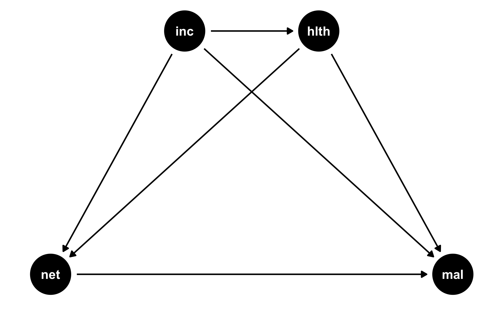
Specify how those nodes are measured.
For the sake of this example, we’ll measure these nodes like so. See the random number example for more details about the distributions.
Malaria risk: scale from 0–100, mostly around 40, but ranging from 10ish to 80ish. Best to use a Beta distribution.
Net use: binary 0/1, TRUE/FALSE variable, where 50% of people use nets. Best to use a binomial distribution. However, since we want to use other variables that increase the likelihood of using a net, we’ll do some cool tricky stuff, explained later.
Income: weekly income, measured in dollars, mostly around 500 ± 300. Best to use a normal distribution.
Health: scale from 0–100, mostly around 70, but ranging from 50ish to 100. Best to use a Beta distribution.
Specify the relationships between the nodes based on the DAG equations.
There are three models in this DAG:
hlth ~ inc: Income influences health. We’ll assume that every 10 dollars/week is associated with a 1 point increase in health (so a 1 dollar incrrease is associated with a 0.02 point increase in health)
net ~ inc + hlth: Income and health both increase the probability of net usage. This is where we do some cool tricky stuff.
Both income and health have an effect on the probability of bed net use, but bed net use is measured as a 0/1, TRUE/FALSE variable. If we run a regression with net as the outcome, we can’t really interpret the coefficients like “a 1 point increase in health is associated with a 0.42 point increase in bed net being TRUE.” That doesn’t even make sense.
Ordinarily, when working with binary outcome variables, you use logistic regression models (see the crash course we had when talking about propensity scores here). In this kind of regression, the coefficients in the model represent changes in the log odds of using a net. As we discuss in the crash course section, log odds are typically impossible to interpet. If you exponentiate them, you get odds ratios, which let you say things like “a 1 point increase in health is associated with a 15% increase in the likelihood of using a net.” Technically we could include coefficients for a logistic regression model and simulate probabilities of using a net or not using log odds and odds ratios (and that’s what I do in the rain barrel data from Problem Set 3 (see code here)), but that’s really hard to wrap your head around since you’re dealing with strange uninterpretable coefficients. So we won’t do that here.
Instead, we’ll do some fun trickery. We’ll create something called a “bed net score” that gets bigger as income and health increase. We’ll say that a 1 point increase in health score is associated with a 1.5 point increase in bed net score, and a 1 dollar increase in income is associated with a 0.5 point increase in bed net score. This results in a column that ranges all over the place, from 200 to 500 (in this case; that won’t always be true). This column definitely doesn’t look like a TRUE/FALSE binary column—it’s just a bunch of numbers. That’s okay!
We’ll then use the rescale() function from the {scales} package to take this bed net score and scale it down so that it goes from 0.05 to 0.95. This represents a person’s probability of using a bed net.
Finally, we’ll use that probability in the rbinom() function to generate a 0 or 1 for each person. Some people will have a high probability because of their income and health, like 0.9, and will most likely use a net. Some people might have a 0.15 probability and will likely not use a net.
When you generate binary variables like this, it’s hard to know the exact effect you’ll get, so it’s best to tinker with the numbers until you see relationships that you want.
mal ~ net + inc + hlth: Finally net use, income, and health all have an effect on the risk of malaria. Building this relationship is easy since it’s just a regular linear regression model (since malaria risk is not binary). We’ll say that a 1 dollar increase in income is associated with a decrease in risk, a 1 point increase in health is associated with a decrease in risk, and using a net is associated with a 15 point decrease in risk. That’s the casual effect we’re building in to the DAG.
Generate random columns that stand alone. Generate related columns using regression math. Consider adding random noise. This is an entirely trial and error process until you get numbers that look good. Rely heavily on plots as you try different coefficients and parameters. Optionally rescale any columns that go out of reasonable bounds. If you rescale, you’ll need to tinker with the coefficients you used since the final effects will also get rescaled.
Here we go! Let’s make some data. I’ll comment the code below so you can see what’s happening at each step.
# Make this randomness consistent
set.seed(1234)

# Simulate 1138 people (just for fun)
n_people <- 1138

net_data <- tibble(
  # Make an ID column (not necessary, but nice to have)
  id = 1:n_people,
  # Generate income variable: normal, 500 ± 300
  income = rnorm(n_people, mean = 500, sd = 75)
) |>
  # Generate health variable: beta, centered around 70ish
  mutate(
    health_base = rbeta(n_people, shape1 = 7, shape2 = 4) * 100,
    # Health increases by 0.02 for every dollar in income
    health_income_effect = income * 0.02,
    # Make the final health score and add some noise
    health = health_base +
      health_income_effect +
      rnorm(n_people, mean = 0, sd = 3),
    # Rescale so it doesn't go above 100
    health = rescale(health, to = c(min(health), 100))
  ) |>
  # Generate net variable based on income, health, and random noise
  mutate(
    net_score = (0.5 * income) +
      (1.5 * health) +
      rnorm(n_people, mean = 0, sd = 15),
    # Scale net score down to 0.05 to 0.95 to create a probability of using a net
    net_probability = rescale(net_score, to = c(0.05, 0.95)),
    # Randomly generate a 0/1 variable using that probability
    net = rbinom(n_people, 1, net_probability)
  ) |>
  # Finally generate a malaria risk variable based on income, health, net use,
  # and random noise
  mutate(
    malaria_risk_base = rbeta(n_people, shape1 = 4, shape2 = 5) * 100,
    # Risk goes down by 10 when using a net. Because we rescale things,
    # though, we have to make the effect a lot bigger here so it scales
    # down to -10. Risk also decreases as health and income go up. I played
    # with these numbers until they created reasonable coefficients.
    malaria_effect = (-30 * net) + (-1.9 * health) + (-0.1 * income),
    # Make the final malaria risk score and add some noise
    malaria_risk = malaria_risk_base +
      malaria_effect +
      rnorm(n_people, 0, sd = 3),
    # Rescale so it doesn't go below 0,
    malaria_risk = rescale(malaria_risk, to = c(5, 70))
  )

# Look at all these columns!
head(net_data)
## # A tibble: 6 × 11
##      id income health_base health_income_effect health net_score net_probability   net malaria_risk_base malaria_effect malaria_risk
##   <int>  <dbl>       <dbl>                <dbl>  <dbl>     <dbl>           <dbl> <int>             <dbl>          <dbl>        <dbl>
## 1     1   409.        61.2                 8.19   63.1      301.           0.369     0              37.9          -161.         45.1
## 2     2   521.        83.9                10.4    83.5      409.           0.684     1              55.0          -241.         23.4
## 3     3   581.        64.6                11.6    73.0      426.           0.735     0              53.0          -197.         36.5
## 4     4   324.        62.0                 6.48   60.6      255.           0.235     0              68.4          -148.         58.7
## 5     5   532.        69.2                10.6    73.4      373.           0.578     1              63.2          -223.         32.7
## 6     6   538.        36.6                10.8    42.6      295.           0.351     0              38.6          -135.         52.5
Verify all relationships with plots and models.
Let’s see if we have the relationships we want. Income looks like it’s associated with health:
ggplot(net_data, aes(x = income, y = health)) +
  geom_point() +
  geom_smooth(method = "lm")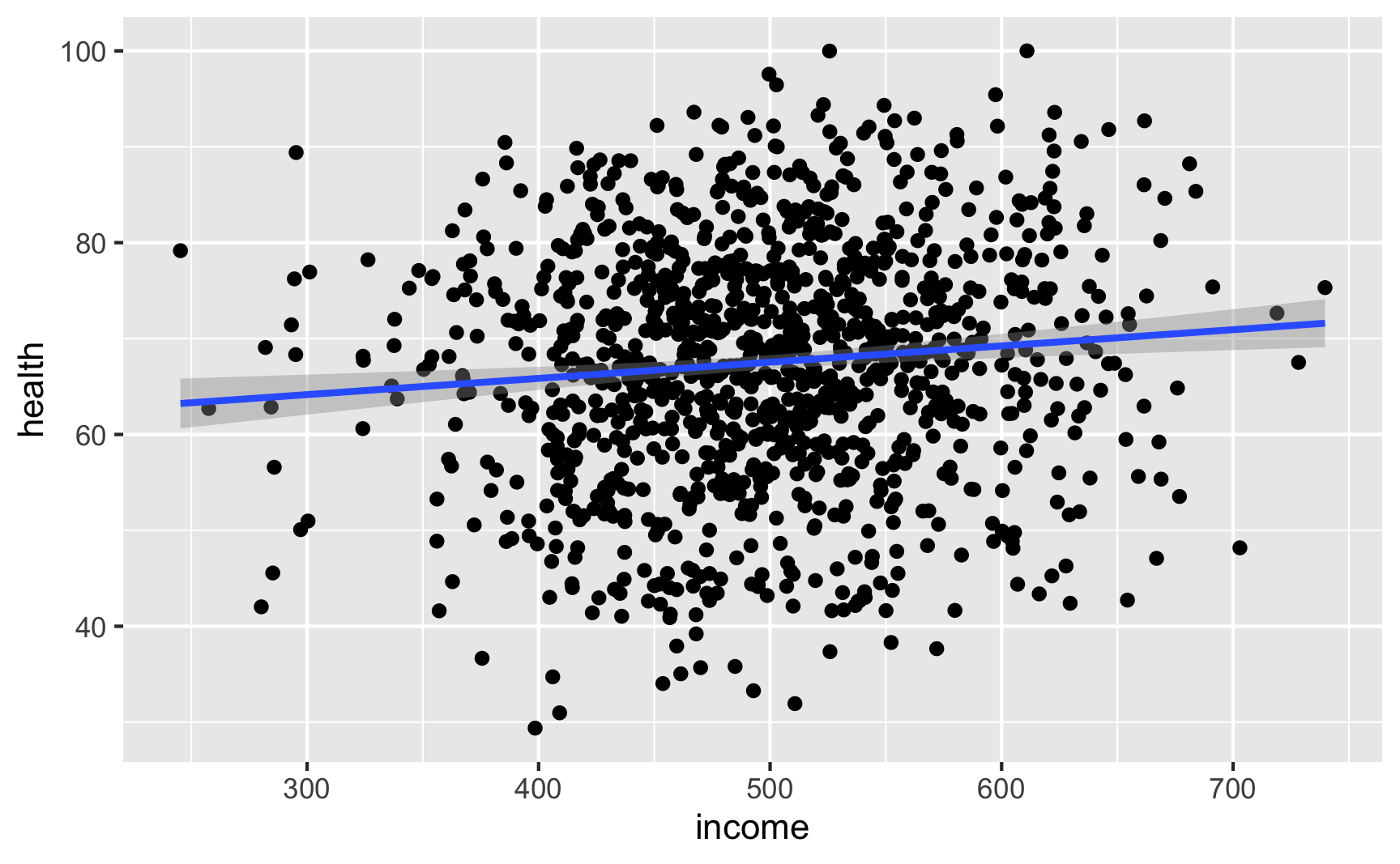
lm(health ~ income, data = net_data) |> tidy()
## # A tibble: 2 × 5
##   term        estimate std.error statistic  p.value
##   <chr>          <dbl>     <dbl>     <dbl>    <dbl>
## 1 (Intercept)  59.1      2.54        23.3  2.24e-98
## 2 income        0.0169   0.00504      3.36 8.15e- 4
It looks like richer and healthier people are more likely to use nets:
net_income <- ggplot(net_data, aes(x = income, fill = as.factor(net))) +
  geom_density(alpha = 0.7) +
  theme(legend.position = "bottom")

net_health <- ggplot(net_data, aes(x = health, fill = as.factor(net))) +
  geom_density(alpha = 0.7) +
  theme(legend.position = "bottom")

net_income + net_health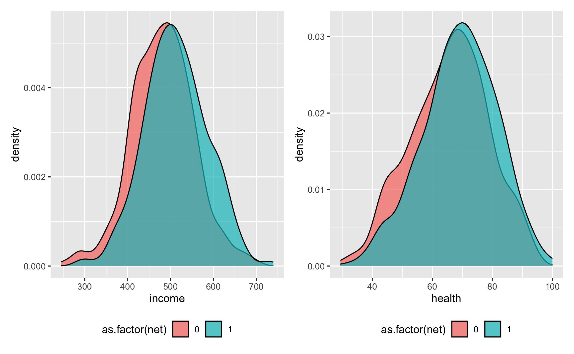
Income increasing makes it 1% more likely to use a net; health increasing make it 2% more likely to use a net:
glm(net ~ income + health, family = binomial(link = "logit"), data = net_data) |>
  tidy(exponentiate = TRUE)
## # A tibble: 3 × 5
##   term        estimate std.error statistic  p.value
##   <chr>          <dbl>     <dbl>     <dbl>    <dbl>
## 1 (Intercept)   0.0186  0.532        -7.49 6.64e-14
## 2 income        1.01    0.000864      6.47 9.93e-11
## 3 health        1.02    0.00491       3.89 9.92e- 5
Try it out!
Is the effect in there? Let’s try finding it by controlling for our two backdoors: health and income. Ordinarily we should do something like matching or inverse probability weighting, but we’ll just do regular regression here (which is okay-ish, since all these variables are indeed linearly related with each other—we made them that way!)
If we just look at the effect of nets on malaria risk without any statistical adjustment, we see that net cause a decrease of 13 points in malaria risk. This is wrong though becuase there’s confounding.
# Wrong correlation-is-not-causation effect
model_net_naive <- lm(malaria_risk ~ net, data = net_data)
tidy(model_net_naive)
## # A tibble: 2 × 5
##   term        estimate std.error statistic   p.value
##   <chr>          <dbl>     <dbl>     <dbl>     <dbl>
## 1 (Intercept)     41.9     0.413     102.  0
## 2 net            -13.6     0.572     -23.7 2.90e-101
If we control for the confounders, we get the 10 point ATE. It works!
# Correctly adjusted ATE effect
model_net_ate <- lm(malaria_risk ~ net + health + income, data = net_data)
tidy(model_net_ate)
## # A tibble: 4 × 5
##   term        estimate std.error statistic   p.value
##   <chr>          <dbl>     <dbl>     <dbl>     <dbl>
## 1 (Intercept)  97.3      1.28         76.1 0
## 2 net         -10.5      0.317       -33.2 1.32e-169
## 3 health       -0.608    0.0123      -49.4 1.25e-284
## 4 income       -0.0320   0.00213     -15.0 1.20e- 46
Save the data.
Since it works, let’s save it:
# In the end, all we need is id, income, health, net, and malaria risk:
net_data_final <- net_data |>
  select(id, income, health, net, malaria_risk)
head(net_data_final)
## # A tibble: 6 × 5
##      id income health   net malaria_risk
##   <int>  <dbl>  <dbl> <int>        <dbl>
## 1     1   409.   63.1     0         45.1
## 2     2   521.   83.5     1         23.4
## 3     3   581.   73.0     0         36.5
## 4     4   324.   60.6     0         58.7
## 5     5   532.   73.4     1         32.7
## 6 6 538. 42.6 0 52.5# Save it as a CSV file
write_csv(net_data_final, "data/bed_nets.csv")